How I wrote a machine learning paper in 1 week that got accepted to International Conference in Machine Learning Applications

December 7, 2022 · 11 min read

How I wrote a machine learning paper in 1 week that got accepted to ICMLA while working full time and raised $8.8 million for OpenBB Terminal.

The open source code is available here.

One year ago, I raised $ 8.8 millions to build OpenBB Terminal full time. But since I was working at a startup in the UK, I had a 3 month notice period.

During that time I worked on documenting pretty much everything I had been working on, BUT that felt short. I felt like the data that came out of our NURVV Run product could be used with a machine learning algorithm in order to detect a foot strike quite efficiently.

So I asked my company:

If I use my spare time to work on this paper will you sponsor me if I get accepted?

My goal was to increase the visibility of our product in academia. And given I spent some time reading papers in the area, I knew that what I had in mind had a shot at working.

My background is not data science, and this was my first time “officially” working on machine learning. I wasn’t 100% sure that my idea would work, but after spending more than 1 year at the company, I knew how the data behaved. I thought I could build an algorithm robust enough to be able to detect a foot strike more efficiently than what others had.

After some time, the company accepted my proposal, and between the time to decide to apply to International Conference on Machine Learning and Applications (ICMLA) and getting ready to start working on the paper, there was 1 week left.

I thought that this window was rather tight given that I had to clean the data, work on the entire code behind the paper from idea to implementation, and write the damn paper. I knew this was gonna be tight, but oh boy. I had one of the harshest weeks of my life. I barely slept for 7 straight days, and skipped the company team event in order to make it through the deadline.

Because of that, I will go into what happened at each step along the way with images. I will skip the cleaning data and boring parts, don’t worry. If you just want to read the final paper, you can find it here: ”Step Detection using SVM on NURVV Trackers”.

Also, if you’ve been following me, you know how much I love open source. Owing to that I open source the code behind the project here.

Exploratory Data Analysis

The Nurvv trackers have an Inertial Measurement Unit (IMU) tracks linear acceleration (accelerometer) and rotational rate (gyroscope). Sometimes it also contains a magnetometer. And Nurvv gave me access to 6 runs from 6 different runners.

My first step was to look into how this data looked. On the left you can see the acceleration (m/s²) and the angular velocity (rad/s).

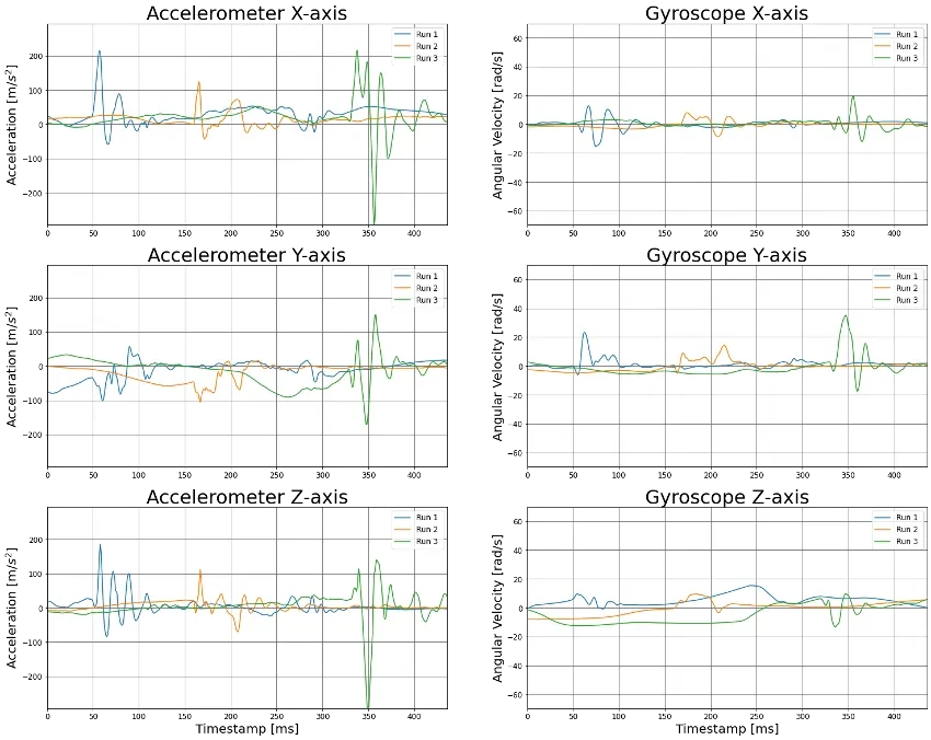
I knew that our IMU had a sampling rate of 1125 Hz (which means that each data point gets sampled at approximately every 888.89μs) and this was critical in order to detect the oscillations that occur when a foot strike occurs (i.e. impact of the foot on the floor makes the IMU oscillate). Thus I zoomed in the zone of impact and used a scatter plot to understand if we were “missing” information.

I found it interesting that the distance between the samples were larger at the time of the impact. So I plotted the IMU accelerometer data and the IMU gyroscope data in a 3D plot interactively as a function of time (below you can see a snapshot).

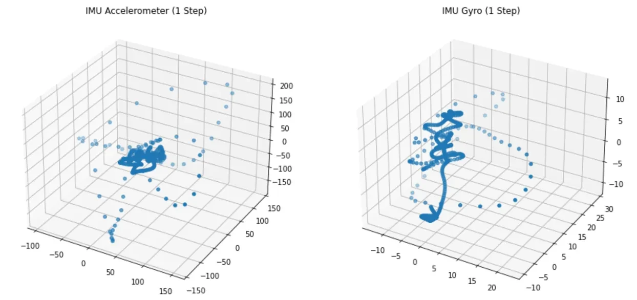
From here it was interesting to note that when the foot is in the air, the samples are somehow concentrated (darker blue), whereas when a step occurs (more sparse) they behave erratically. The plot above was snapshotted with 3 steps that occurred.

From that 3D plot I had the intuition that by utilizing a principal component analysis (PCA)**, I could reduce the dimensionality without losing much information. The result is shown below,

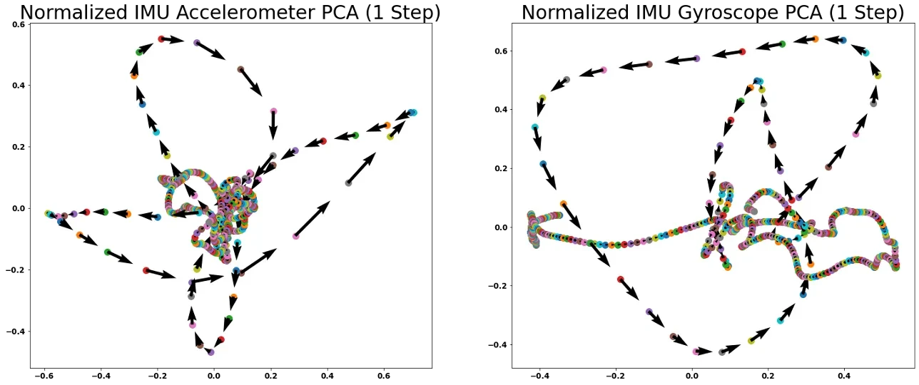
This made me think that I could use a support vector machine (SVM) in order to detect whether a foot strike has occurred or not. And what I was most excited about it was:

This model isn’t time-dependant. Meaning that it would be fascinating to be able to predict whether a step occurred or not without the notion of time, but the current IMU data.
We can develop an SVM model for each runner style. Then create an ensemble model with hard voting which allowed for the model that has seen more similar data, to be more confident in the classification of foot strike vs not foot strike.

But this was all a theory, I needed to prove it.

The first issue I had was: SVM is a supervised learning model. This meant that for the sampling data I was providing the model, I would have to classify whether those samples corresponded to a foot strike or not.

The issue? Although the product had force sensitive resistors (FSR) in the insoles, I didn’t have access to the samples that corresponded with these IMU samples.

So I knew that I would have to classify the data myself. Manually would have been a nightmare and not reliable enough, so I needed to build an algorithm that could classify the data quite reliably. Signal processing theory, here I go.

Labelling data for a supervised learning problem

Get the raw IMU samples (accelerometer and gyroscope)
Do the difference in magnitude between the accelerometers samples and then the gyroscope samples
Apply root sum squared to the magnitude difference of accelerometer data, and then similarly to gyroscope data
Standardize the accelerometer data and the gyroscope data. This is so the data can be somehow compared with each other since the magnitude varies as one represents linear acceleration and the other angular rate.
Do the average between these 2 signals. This makes the data more robust.
Finally, apply a convolution to the resulting signal with a rectangular pulse. This allows to remove “drops” from the signal and ensures a smoother signal.

Below you can see the formulas and signal changes that were made in order to obtain the final result:

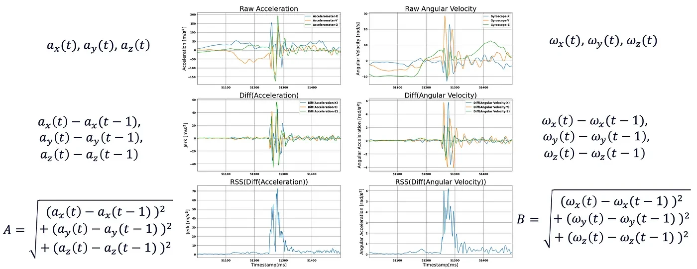
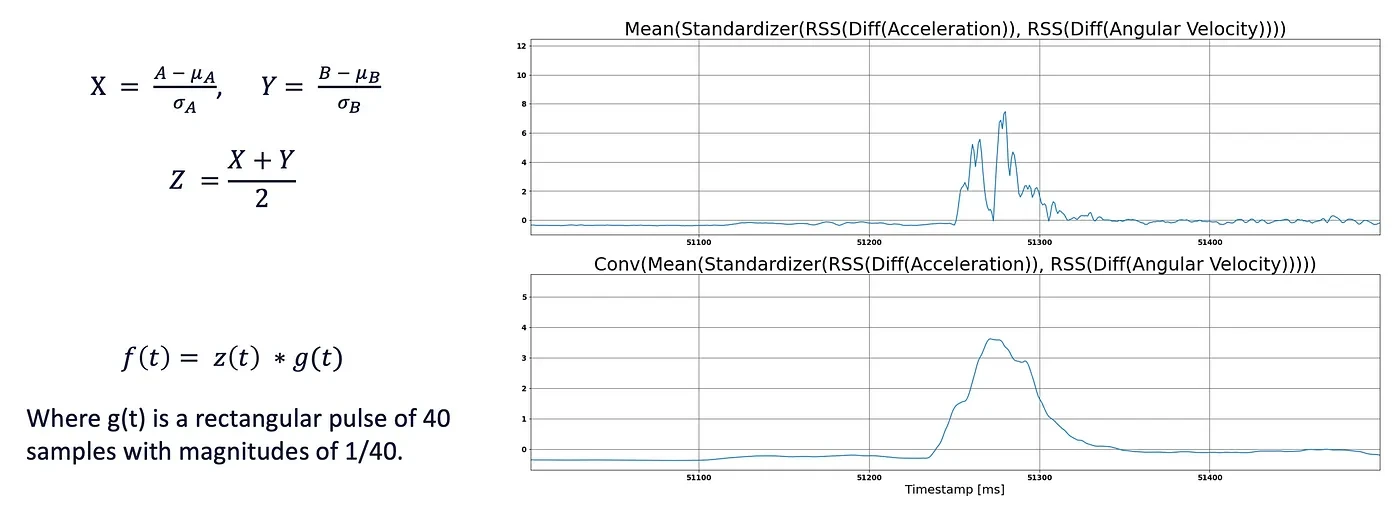
After this, I selected a sensible value of 0.3 to be used as a threshold on the resulting signal to classify step vs no-step.

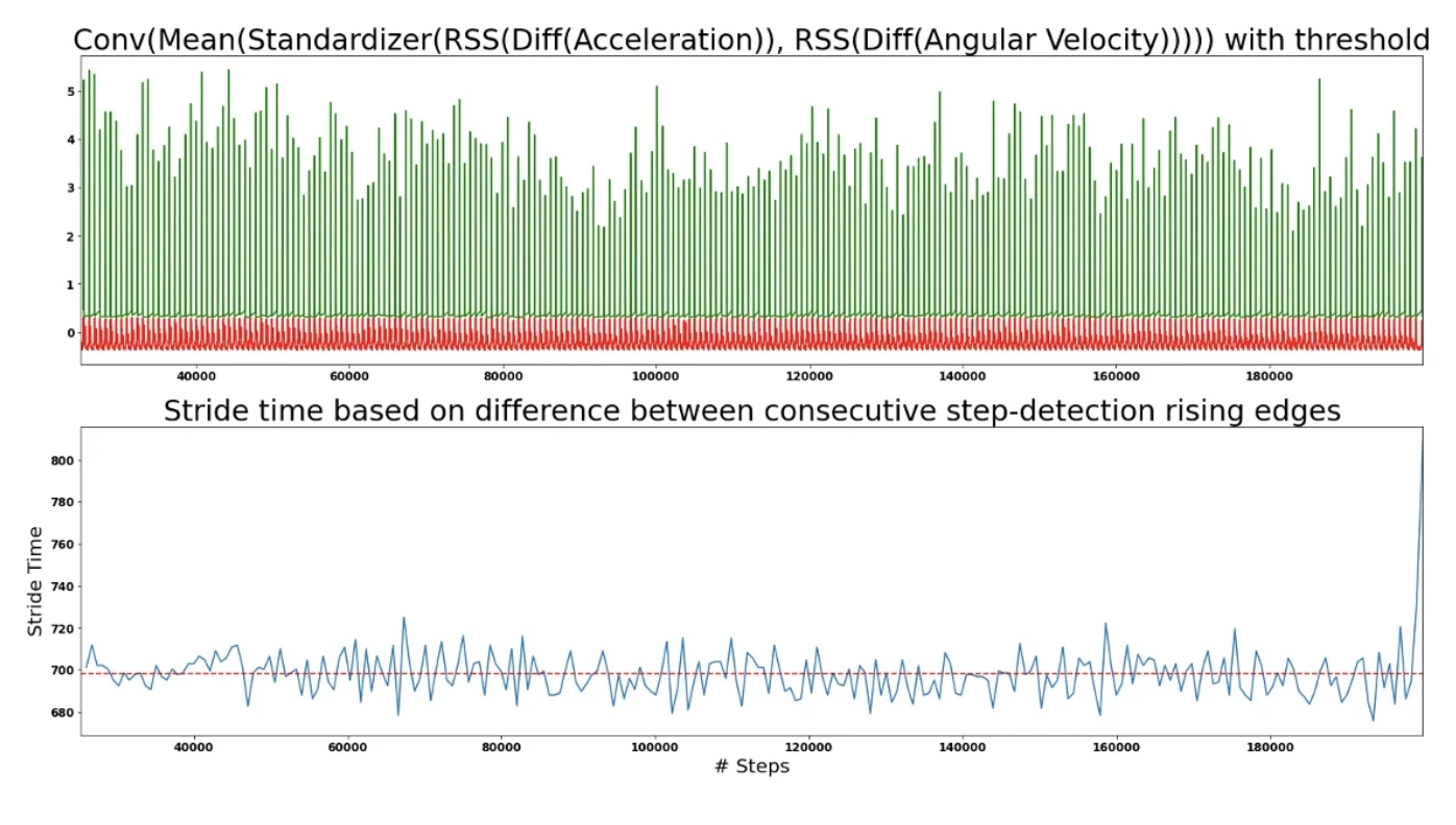
I applied the difference between each first foot strike detected in order to make sure that there was no missed step. As you can see above the stride time is around 700ms which is what is expected of a runner jogging.

Someone might be wondering; If this gives such a great result, why did I need machine learning in the first place? The reason is because standardization and convolution (steps 4 and steps 6) are a post-processing signal technique. Therefore, it cannot be deployed in running time, and relies on data that happens in the future.

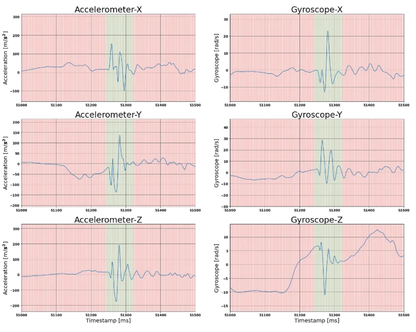
For illustration purposes, here is how the initial raw IMU data behaves against the labelling from signal processing approach (red background means no step, while green background means step).

Support Vector Machine for classification

For the model, SVM was selected because:

It works well with high dimensional data (6 IMU samples) because it only uses a few of these points (called support vectors) to create this hyperplane (decision boundary) between classes.
SVM is ideal for binary classification problems.
RBF kernel allows to handle non-linear data.

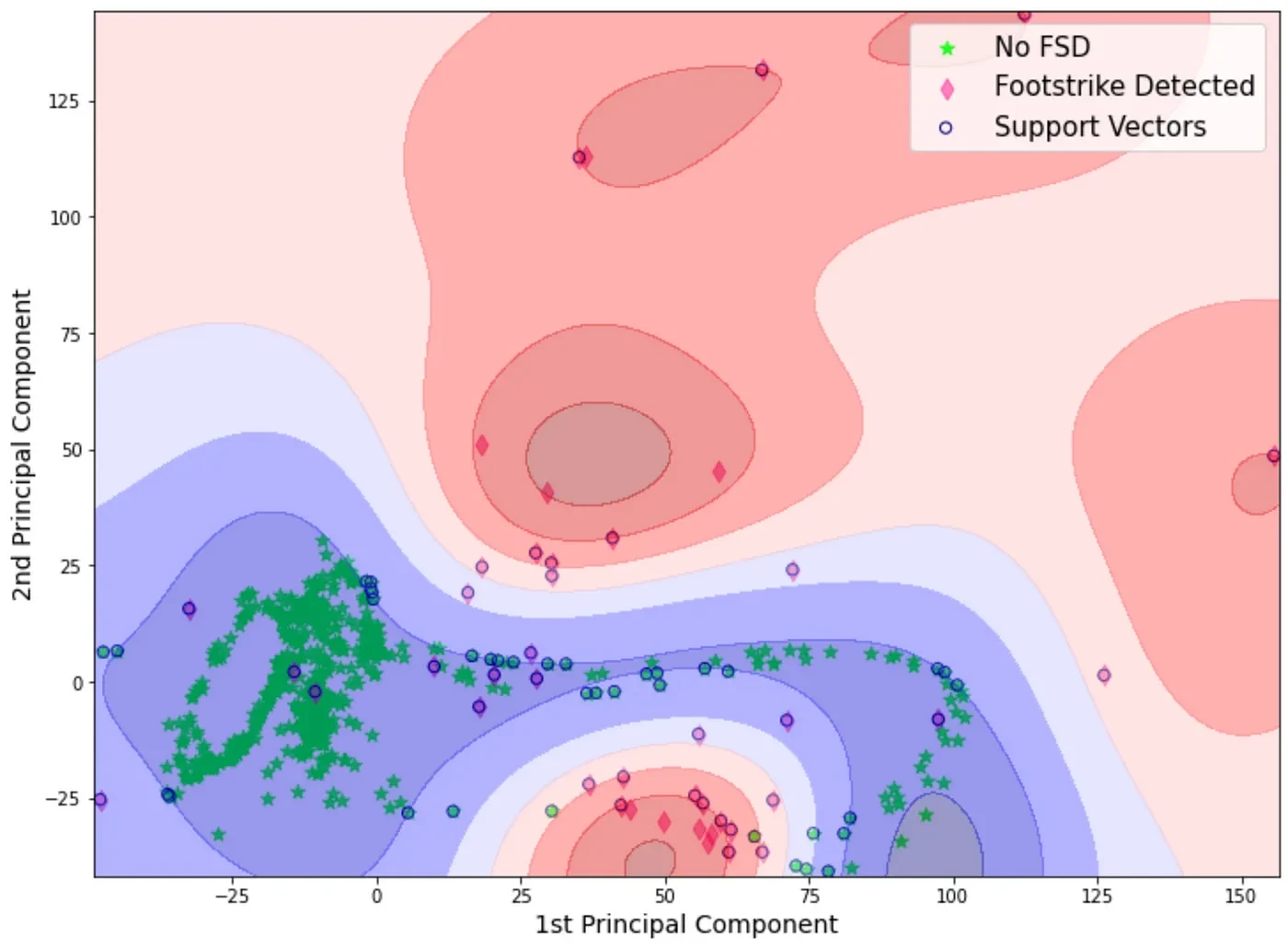
This is the type of classification that SVM is capable of (this is the raw acceleration data with a PCA applied, and the SVM classification on the background for a model that was trained using that same data).

C and gamma hyperparameters

Given each dataset is rather large to perform grid search optimization on C and gamma, a subset of each of the datasets is used to extract these parameters.
Each dataset subset is now split: 80% for training data and 20% for validation.
Thus, 80% of the data subset is used to apply SVM with different combinations of C and gamma over a 2D grid. The remaining 20% is used to test the logistic loss and assess optimal hyperparameters.

Training and testing

80% of data is used for training and 20% is used for testing.
Although the testing is done out-of-sample, given the nature of the data (where it comes from the same distribution) it is almost as if it was an in-sample.
In our case this is ideal as we want each model to perform very well on its own dataset. We want each model to generalize well for that very specific type of data (runner style, speed and terrain).
A 5-sample moving average is applied before assessing the classification of our model, this is to remove spurious samples. A small window needs to be selected to not introduce a delay in the recognition of a step.
Since our data set is imbalanced (i.e. there are more samples being no-step than step samples) we’ll use Geometric Mean (G-Mean) evaluation score, since this measure tries to maximize the accuracy on each of the classes while keeping their accuracies balanced.

Result

In the same dataset where we trained our SVM, we were able to achieve a G-Mean of 0.9645. This is rather expected since this is a powerful model and it was trained on that same data.

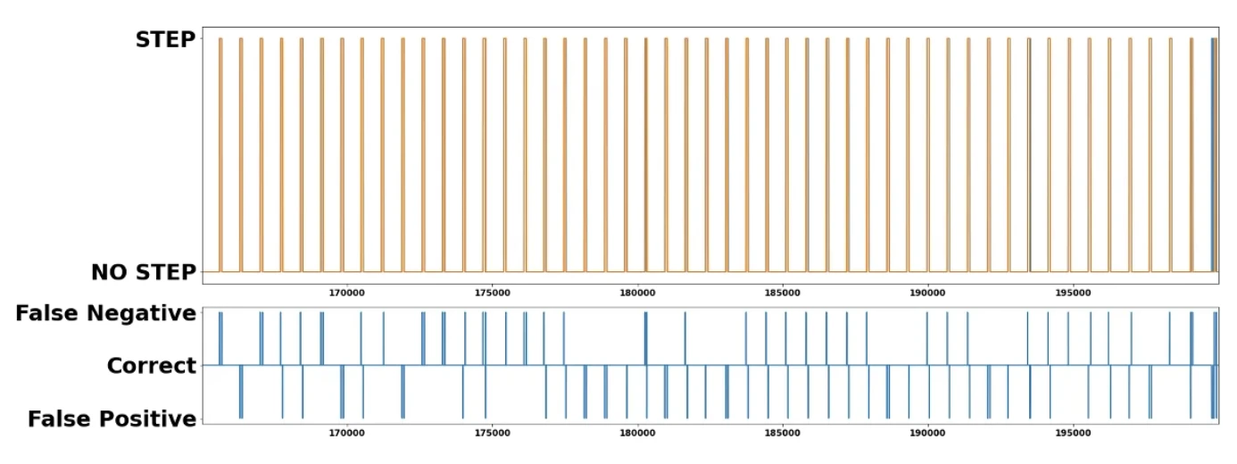
From the graph above this result is very positive given that the mislabelling always occurs at the boundary of a step / no-step detection. And since the sampling occurs very fast, we have some margin of error.

Ensemble SVM model architecture

This model as expected had a poor performance in an unseen dataset. This is normal as the data came from a different runner, running at a different speed in a different terrain. Thus, in order to create a more robust model, we built this ensemble SVM model architecture.

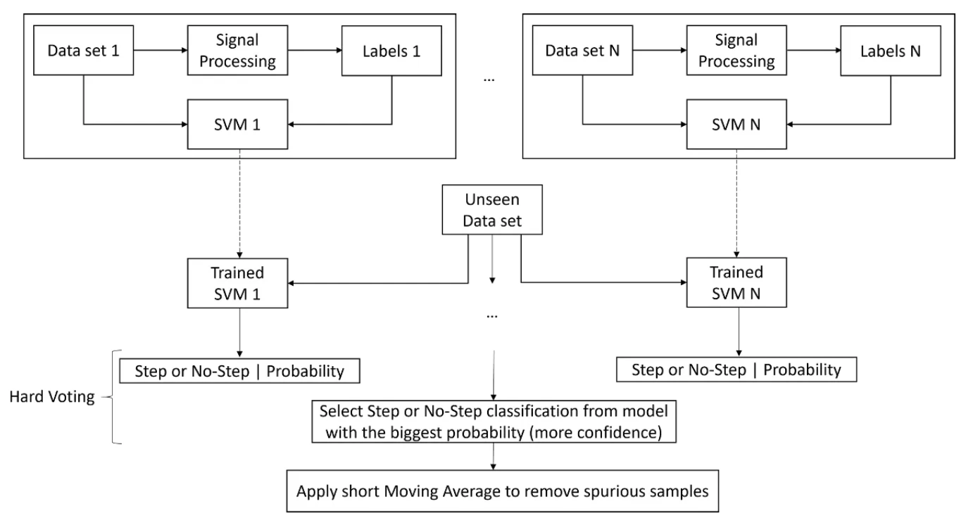
Each dataset has the signal processing technique applied in order to obtain the labelling. With this labels, an SVM model can be trained.

Then, an unseen dataset (not used for training) will be used as input for all the trained SVM models. I.e. each input (3 accelerometer samples and 3 gyroscope samples) will be given to each SVM model which will output 0 or 1 to denote no-step or step, respectively.

My rationale there was: I could do a major voting approach, BUT because of how I trained the data. It could happen that one of the models had the sample being very inside the boundary, whereas 2 others had it just outside, and the later would win. This is not what I was looking for.

Because of this boundary approach associated with SVMs, I knew that although SVM doesn’t provide probability estimates directly, these could be calculated. So I took advantage of that. And used that probability estimate to select whether the input was considered a stop or not. My rationale was: the model that has seen more similar IMU samples is likely to have a higher confidence in their output and as output they will have what I provided as a label in advance.

Finally, I applied a 5-sample moving average to the step (1) / no-step (0) output and round the value to be classified as step and no-step. This allowed to remove spurious samples.

Results

The prediction for a single SVM was extremely accurate because the model was trained on data samples from that same run (i.e. distribution). On the other hand, the ensemble prediction didn’t run on data from that distribution, hence, making this problem much more complex. However, even with that constraint, a G-Mean of 0.8756 was still achieved.

Future work

Employ the data coming from the ”smart” insoles as an alternative ground-truth for determining step versus no-step conditions.
The diversity of the data set can also be expanded to account for more surfaces, running speeds and styles.
Explore whether the characteristics of the PCA plot of IMU data can be used to categorize different running styles.
The exploration of different classification algorithms for the step detection problem, e.g. applying a long-short term memory (LTSM) neural network algorithm to exploit the time-dependency between samples.
Implement this proof-of-concept code on the production NURVV Run system, to test the prediction technique in a real-life scenario and consider computational time.

Final remarks

This was my first most technical blogpost where I went into details in how I wrote a ML paper that was accepted in a major conference in 1 week. Would love to know your thoughts on it.

Feel free to check the full paper version here: https://ieeexplore.ieee.org/abstract/document/9680024